The Neural Network at its Simplest

Neural Networks:

Neural Network is a branch of machine learning branch under reinforcement domain, which is used in prediction of any variable from given raw data through network like structure.Neural Network’s structure is most likely to be human neural system.

Here it got nucleus at the center part and dendrites for electrical signal receiving and axon for signal passing and axon terminals for signal output for dendrites of another neuron.

x = input

h = output

a = hidden layers

b = bias factor

w = weights

Perpectron:

Here “x” is input variable with some values and every input nodes are connected to the hidden layer where the summation of the input with their respective weights are done and lastly the bias factor is added.Further “Activation Function” is added to take the output “y” hat.

The weight’s value varies from 0 to 1 according to the impact of that particular node on output, In initial stage the weights are randomly initialized and later it will get adjusted accordingly.

The Activation Function decides whether the node should be activated or not depending upon the sum of input variable with bias. The activation function is applied to hidden layer and output layer.

Some of Activation Functions are Threshold Activation Function, Sigmoid Activation Function, Tangent Hyperbolic Activation Function, Rectifier Activation Function and many more.

Here there will be some decided value is set, the values above will be set high or activate the node and value below will be set low or deactivate the node.

Threshold Activation Function:

It is also called as Binary Function.

Sigmoid Activation Function:

It is used most in the probabilistic cases.

Rectifier Function(ReLU):

ReLU is the most commonly used in most of the ANNs.

Forward Propagation:

As the name suggests the Forward propagation is the forward data flow network, As here the data is fed at input layer and further it is carried out to the hidden layers. The processing of the input variables in hidden layer is done according to activation function applied to that node and later it carried forward to output layer where output will be taken according to the activation function.

Note: The network where the data only flows in forward direction is called Feed Forward Network. No backward flow is possible in Feed Forward Network.

Loss Function:

It defines the performance of the model. And it is done by the calculation of the difference between actual output and predicted output in the real number value. Lower the Loss Value of the model higher the precision of model.

The Loss Value can be taken in three ways, some are taken by whole set’s value at once as Gradient Descent, Or once in every single point of dataset as Stochastic Descent, or by dividing the whole set as some N number of divisions as Mini-Batch Stochastic Descent.

Setting of the weights accordingly to the impact on neurons will reduce the Loss Function.

Back Propagation:

Back Propagation is same as Forward Propagation but with coming backward of network too. Back Propagation is simply we can say Feedback in Neural Networks because back propagation is just an error calculation output value.

The Error value of Neural Network is simply calculated by the difference between the network’s output and desired output.

Error = Actual Output — Desired Output

The calculated error value is used in back propagating which means going back to the all neurons of the hidden layers from output layer to adjust the weights assigned to it for minimizing the error in output and to get the desired output or closer value.

Gradient Descent:

Gradient Descent is an intensively used algorithm for optimization the neural network model’s parameters such as coefficients and weights. Considering the 2D graph,

The Gradient Descent is just getting down to that minimum cost value/ loss value, this is done by calculating the slope of the point’s derivative and point is said to be at minimum value when slope is zero(slope pointing downward is negative and pointing up is positive) and learning rate Using this algorithm reduction of cost function is done where right learning rate has to be set to reach the graph’s minimum value.

Stochastic Gradient Descent:

Though the Gradient Descent is great but its slow and high computational algorithm which takes a lot of time to execute. To improve the speed of the algorithm it is evolved as Stochastic GD it’s just the same but calculation is done on every single point which is actually faster because it uses multiple threads at the same time for execution

Another use of Stochastic Gradient is its way efficient in finding global minima out of several minimums.

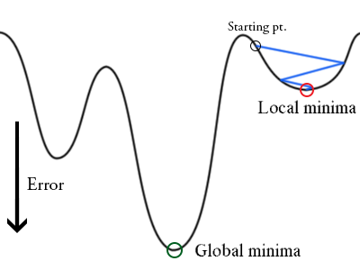
Sometimes there are alot of minimums(local minima) in the cost functions but there would be one global minimum value(least value of cost function) out of the whole graph. And proper learning rate will shoot the point to global minima. Again it’s not completely sure that only global minimum.

Cost Function graph in 3D

Mini Stochastic Gradient Descent:

Mini SGD is the Stochastic GD only but the error calculation is done in batches(set of data points out of whole) not like calculation for every point. This is better than normal SGD because it’s less in computational factors because it uses less threads than SGD.